Lecture Newcastle Text analysis
In the past one decade, there has been an exponential surge in the online activity of people across the globe. The volume of posts that are made on the web every second runs into millions. To add to this, the rise of social media platforms has led to flooding to content on the internet.
Social media is not just a platform where people talk to each other, but it has become very vast and serves many more purposes. It has become a medium where people
- Express their interests.
- Share their views.
- Share their displeasures.
- Compliment companies for good and poor services.
So in this lecture, we are going to learn how we can gather, analyze and present what users are posting on Twitter to come up with insight for Policy communication strategies or other types of Public health strategies.
1. Apply for a Twitter Developer Account
You’ll need a Twitter Developer account since it gives you access to a personalized API key, which we will need later on. This key is unique to every account, so you mustn’t share it.
Visit Twitter Developer and create an account. You can use the same login credentials to your personal Twitter account if you’d like.
You will need to apply for an account, so make sure to follow the steps. It may take some time to set up the account, as there are a few questions you’ll need to answer. Most questions require a decent amount of input, so answer it to the best of your ability. How to create the Twitter app?
Twitter has made the task of analyzing tweets posted by users easier by developing an API which people can use to extract tweets and underlying metadata. This API helps us extract twitter data in a very structured format which can then be cleaned and processed further for analysis.
To create a Twitter app, you first need to have a Twitter account. Once you have created a Twitter account, visit Twitter’s app page and create an application.
2. Create a Twitter API App
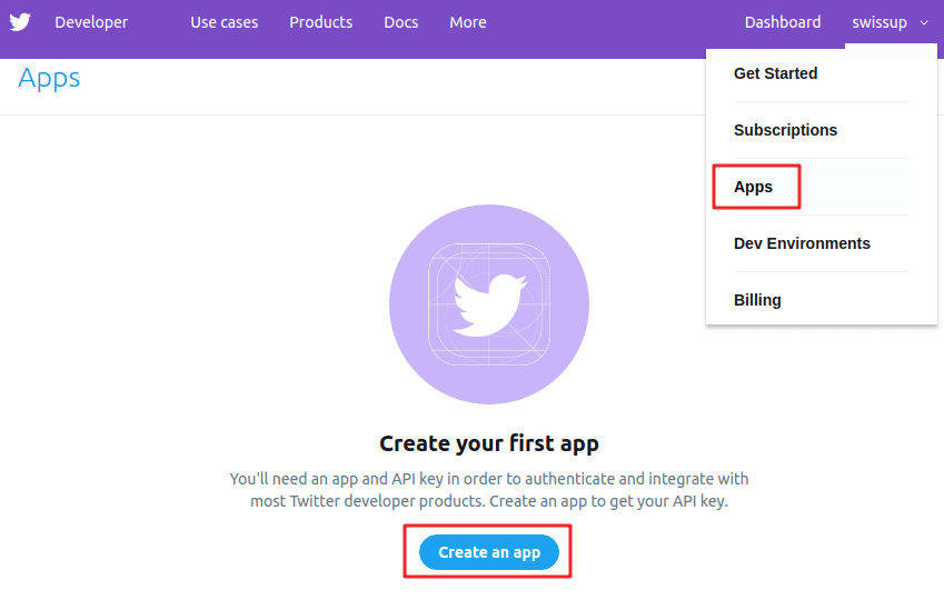
It could take some time to get approved for a Developer account. However, after the approval, look at the top right of the navigation bar and select apps to create an app that is part of generating an API key.
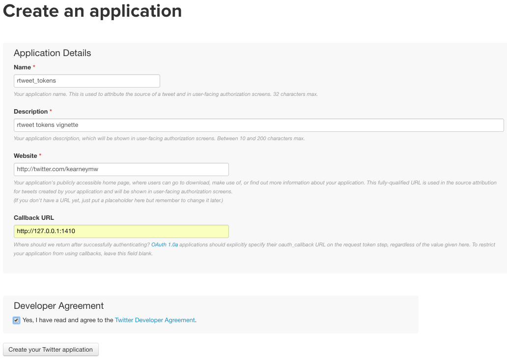
2.1 Complete the fields (important: Callback URL must be exact)
- Name: {{initials}}_twitter_app
- Description: {{something about analyzing Twitter data}}
- Website: https://twitter.com/{{you_screen_name}}
- Callback URL: http://127.0.0.1:1410
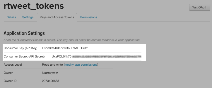
2.2 Copy the keys
- 2.3 Click Create your Twitter application
- 2.4 Select Keys and Access Tokens tab
- 2.5 Copy the Consumer Key (API Key) and Consumer Secret (API Secret) and paste into R script
copy and pasted your keys (these are fake)
consumer_key <- "XYznzPFOFZR2a39FwWKN1Jp41"
consumer_secret <- "CtkGEWmSevZqJuKl6HHrBxbCybxI1xGLqrD5ynPd9jG0SoHZbD"
If you’re lost, this is a great video for the API key.
Now that you’re all set up, let’s get started in R Studio!
3. Let’s start with the programming steps

Load packages in the R enviorament
library(rtweet)
library(tidyverse)
library(purrr)

library(lubridate)
library(DataExplorer)

library(kableExtra)
library(scales)
library(ggridges)
library(DT)
3.1 Pull Tweets
Now that all the steps for setting up the twitter API are done, we can now gather tweets. Let’s breakdown the function below.
api_key <- "xxxx"
api_secret_key <- "xxxx"
access_token <- "xxxxxx"
access_token_secret <- "xxxx"

# authenticate via web browser
token <- create_token(
  app = "Accademic",
  consumer_key = api_key,
  consumer_secret = api_secret_key,
  access_token = access_token,
  access_secret = access_token_secret)
Search tweets or users
In this example we search for 5000 tweets containing #covid, the common hashtag used to refer at the covid19 outbreak, including the in English language:
rt <- search_tweets("#covid", n = 5000, include_rts = TRUE, fileEncoding = "UTF-8", lang = "en")Twitter rate limits cap the number of search results returned to 18,000 every 15 minutes. To request more than that, set retryonratelimit = TRUE and rtweet will wait for rate limit resets for you. For more details about the Twitter’s API package (rtweet) visit the page https://github.com/ropensci/rtweet where all the details to gather tweets are provided!
For those who want to code alongside, there is available the dataset used for the following tutorial on my GitHub page. Download the dataset and upload it to use the code and get the same results
Load the dataset
library(readxl)

df <- read_excel(".. //df_Covid_Newcastle.xlsx")
Exploring tweets
Have a quick look at the some of the gathered variables like the tweets text, the time and the likes recived.
ddf <- df %>%
  select(user_id, text, created_at, favorite_count)

datatable(ddf)
Timeline of tweets
The ts_plot() function from the rtweet package enables us to plot the frequency of tweets over a variety of time intervals (e.g. “secs”, “mins”, “hours”, “days”, “weeks”, “months”, “years”)
df %>%
  ts_plot("30 minutes") +
  ggplot2::theme_minimal() +
  ggplot2::theme(plot.title = ggplot2::element_text(face = "bold")) +
  ggplot2::labs(
    x = NULL, y = NULL,
    title = "Frequency of #Tweets",
    subtitle = "Twitter status (tweet) counts aggregated",
    caption = "\nSource: Data collected from Twitter's REST API via rtweet")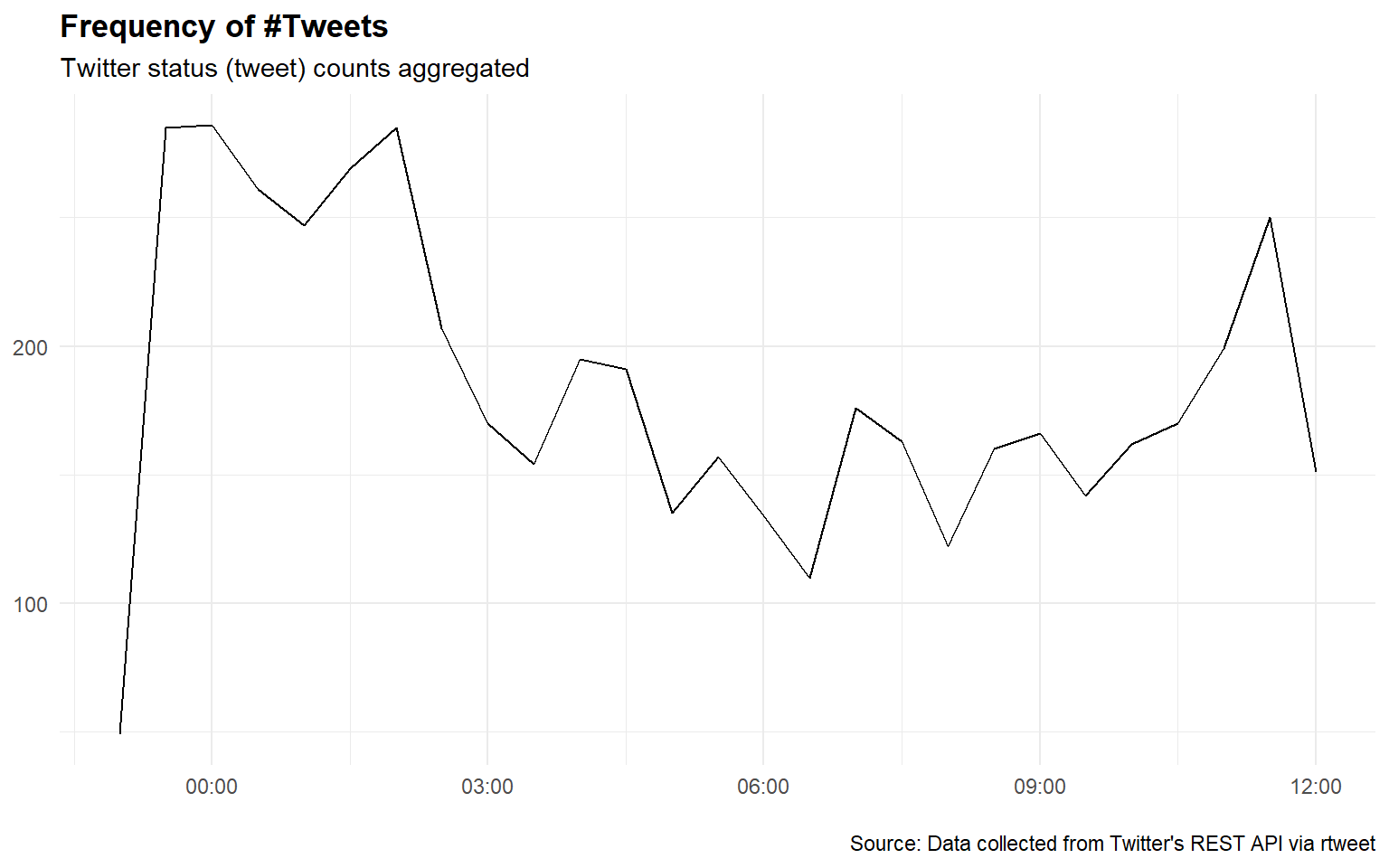
Most re-tweeted tweets
The Twitter API helpfully returns a “retweet_count” variable whose values can easily be sorted. Here we sort all the tweets in descending order by the size of the “retweet_count”, slice off the top row and print the date, handle, text and retweet count.
df %>%
  filter(is_retweet == F) %>%
  arrange(desc(retweet_count)) %>%
  select(user_id, text, retweet_count)
## # A tibble: 1,072 x 3
## user_id text retweet_count
## <chr> <chr> <dbl>
## 1 18831926 "EXCITING—The Novavax protein-based #COVID~ 795
## 2 1426748894751297537 "#COVID DISINFORMATION ALERT\r\n\r\nClaim:~ 199
## 3 1375470391 "What concerns me the most is 8-10 months ~ 183
## 4 1403201252910059522 "#CDC also known as #Pfizer and #Moderna a~ 98
## 5 275104144 "Read this article: #WhiteAmericans at end~ 59
## 6 811826520 "Longest lockdowns in the world, 800 dead,~ 46
## 7 243983947 "Just days after #XiJinping said there’s t~ 45
## 8 1375470391 "Why are so many people still vocal about ~ 38
## 9 822496079274975232 "Crises create opportunity for durable cha~ 34
## 10 1094971056358637568 "Exactly one year, when New Zealand was st~ 26
## # ... with 1,062 more rowsTop emoji
To identify the most used emoji we can use the ji_extract_all() function from the emo package. This function extracts all the emojis from the text of each tweet. We can then use the unnest() function from the tidyvers package to split out the emojis, count, sort in descending order and identify the top 10
library(emo)

df_emo <-df %>%
  mutate(emoji = ji_extract_all(text)) %>%
  unnest(cols = c(emoji)) %>%
  count(emoji, sort = TRUE) %>%
  top_n(10)
## Selecting by ndatatable(df_emo)Top mentions
Here we tokenise the text of each tweet and use str_detect() from the stringr package to filter out words that start with an @ .
library(tidytext)

df %>%
  unnest_tokens(mentions, text, "tweets", to_lower = FALSE) %>%
  filter(str_detect(mentions, "^@")) %>%
  count(mentions, sort = TRUE) %>%
  top_n(10)
## # A tibble: 10 x 2
## mentions n
## <chr> <int>
## 1 @CDCgov 214
## 2 @CDCDirector 203
## 3 @jimsciutto 54
## 4 @WHO 44
## 5 @AlboMP 41
## 6 @nytimes 34
## 7 @DHSCgovuk 24
## 8 @kidneycareuk 24
## 9 @LeukaemiaCareUK 24
## 10 @marieevemo 244. Text Analysis
As we stated above, we define text analysis as being machine learning technique used to automatically extract valuable insights from unstructured text data. Analyst can use text analysis tools to quickly digest online data and documents, and transform them into actionable insights. Structuring text data in a tidy format means that it conforms to tidy data principles and can be manipulated with a set of consistent tools https://www.tidytextmining.com/index.html.
4.1 Text analysis per words x day
library(tidytext)

rt_words <- df %>%
  select(user_id, text, retweet_count, favorite_count, created_at) %>%
  unnest_tokens(word, text, token = "tweets") %>%
  anti_join(stop_words, by = "word")

# Count the frequency of the most used words
rt_words %>%
  count(word, sort = T)
## # A tibble: 9,892 x 2
## word n
## <chr> <int>
## 1 #covid 4750
## 2 people 1498
## 3 vaccine 879
## 4 #covid19 799
## 5 covid 784
## 6 pfizer 779
## 7 booster 749
## 8 #booster 720
## 9 receive 712
## 10 18 709
## # ... with 9,882 more rowsTop tweets sorted by the average retweet and likes received
rt_words %>%
  group_by(word) %>%
  summarise(n = n(),
            avg_retweets = mean(retweet_count),
            avg_favorite = mean(favorite_count)) %>%
  filter(n >= 100)
## # A tibble: 144 x 4
## word n avg_retweets avg_favorite
## <chr> <int> <dbl> <dbl>
## 1 #ba5 695 795. 3.85
## 2 #booster 720 767. 3.73
## 3 #cdc 139 35.3 3.53
## 4 #coronavirus 135 3.97 0.689
## 5 #covid 4750 4282. 1.67
## 6 #covid19 799 49.9 1.82
## 7 #covidisnotover 254 126. 4.03
## 8 #covidisntover 241 160. 1.51
## 9 #longcovid 158 610. 0.930
## 10 #novavax 708 780. 3.78
## # ... with 134 more rowsTop 5 most retweet tweets
df_rtw <-df %>%
  filter(is_retweet == F) %>%
  arrange(desc(retweet_count)) %>%
  select(user_id, text, retweet_count) %>%
  top_n(5)

datatable(df_rtw)
5. Sentiment analysis
When human readers approach a text, we use our understanding of the emotional intent of words to infer whether a section of text is positive or negative, or perhaps characterized by some other more nuanced emotion like surprise or disgust. We can use the tools of text mining to approach the emotional content of text programmatically, as shown in Figure
One way to analyze the sentiment of a text is to consider the text as a combination of its individual words and the sentiment content of the whole text as the sum of the sentiment content of the individual words. The tidytext package provides access to several sentiment lexicons, nd in particular the syuzhet allows the use of several lexicons for the emotions measurement like:
AFINN from Finn Årup Nielsen, bing from Liu and collaborators, and *nrc from Saif Mohammad and Peter Turney
5.1 Specific sentiment lexicons
library(syuzhet)
library(ggplot2)
library(scales)
library(reshape2)
library(tm)

mySentiment <- get_nrc_sentiment(df$text)
df <- cbind(df, mySentiment)
sentimentTotals <- data.frame(colSums(df[,c(57:66)]))
names(sentimentTotals) <- "count"
sentimentTotals <- cbind("sentiment" = rownames(sentimentTotals), sentimentTotals)
rownames(sentimentTotals) <- NULLPlot the Sentiment analysis
Let’s look at the sentiment scores for the eight emotions from the NRC lexicon in aggregate for all my tweets. What are the most common emotions in my tweets, as measured by this sentiment analysis algorithm?
ggplot(data = sentimentTotals, aes(x = sentiment, y = count)) +
  geom_bar(aes(fill = sentiment), stat = "identity") +
  theme(legend.position = "none") +
  xlab("Sentiment") + ylab("Total Count") + ggtitle("Total Sentiment Score for All Tweets")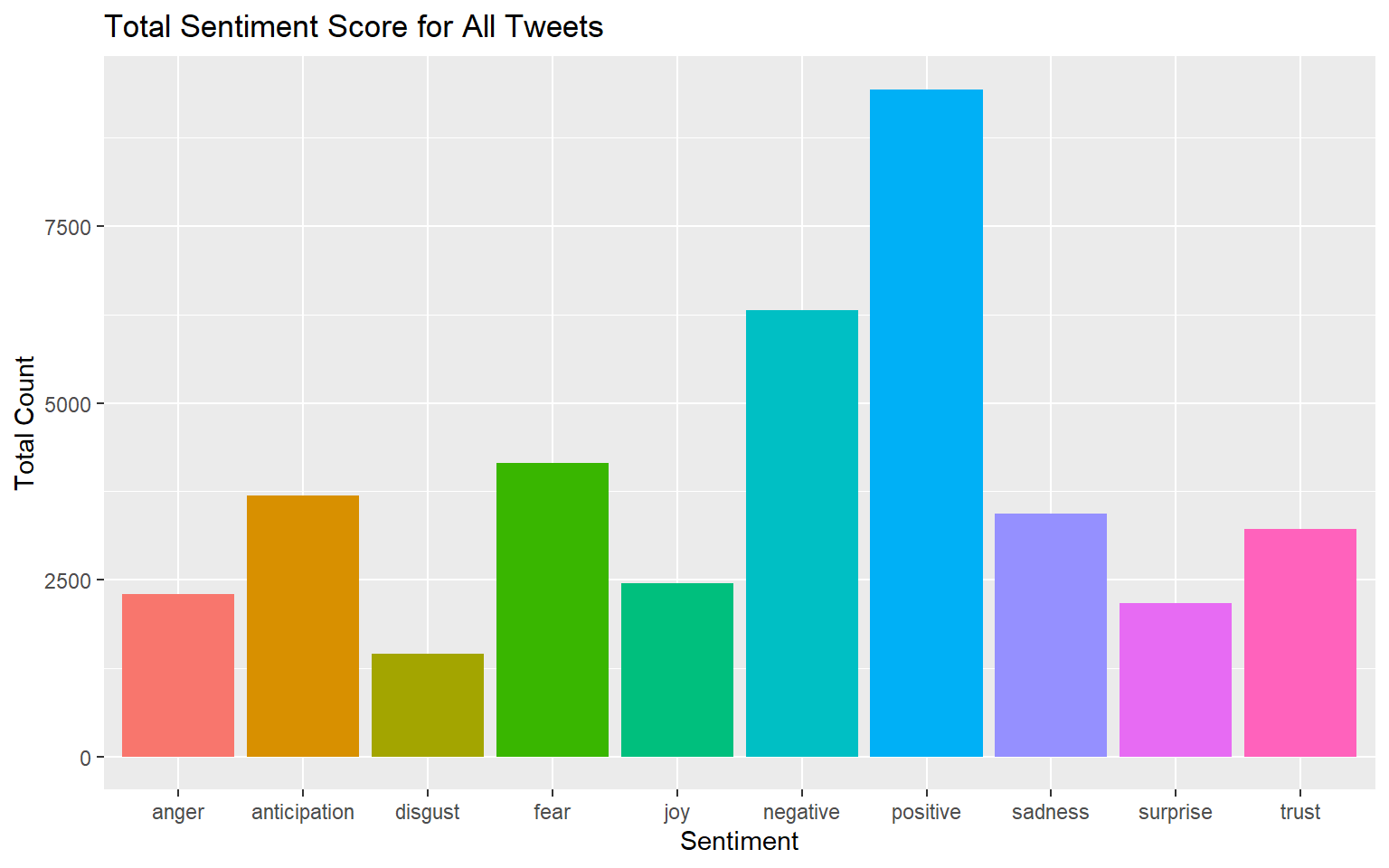
6. Topic modeling
Topic modeling is a methodology for unsupervised classification, similar to the clustering methods numeric data, which finds natural groups of items across a set of documents. Topic Modeling is used to discover “latent” topics in a given selection of documents. Topic models are particularly common in text mining to unearth hidden semantic structures in textual data.Topic models are also referred to as probabilistic topic models, which refers to statistical algorithms for discovering the latent semantic structures of an extensive text body One of the most popular topic models is latent Dirichlet allocation (LDA) Blei et al. 2003.
LDA is a particularly popular method for fitting a topic model. It treats each document as a mixture of topics, and each topic as a mixture of words. This allows documents to “overlap” each other in terms of content, rather than being separated into discrete groups, in a way that mirrors typical use of natural language.

Ok.. LDA is not the easiest thing to understand at first glance…

Without diving into the math behind the model, we can understand it as being guided by two principles.
Every document is a mixture of topics. We imagine that each document may contain words from several topics in particular proportions. For example, in a two-topic model we could say “Document 1 is 90% topic A and 10% topic B, while Document 2 is 30% topic A and 70% topic B.”
Every topic is a mixture of words. For example, we could imagine a two-topic model of American news, with one topic for “politics” and one for “entertainment.” The most common words in the politics topic might be “President”, “Congress”, and “government”, while the entertainment topic may be made up of words such as “movies”, “television”, and “actor”. Importantly, words can be shared between topics; a word like “budget” might appear in both equally.
6.1 Cleaning and processing the text data
The first step is Clean the Text
df$text <- tolower(df$text) # Make everything consistently lower case
df$text <- gsub("http.+ |http.+$", "", df$text) # Remove links
df$text <- gsub("[[:punct:]]", "", df$text) # Remove punctuation
df$text <- gsub("[ |\t]{2,}", "", df$text) # Remove tabs
df$text <- gsub("amp", "", df$text)# "&" is "&"after punctuation removed
df$text <- gsub("^ ", "", df$text) # Leading blanks
df$text <- gsub(" $", "", df$text) # Lagging blanks
df$text <- gsub(" +", " ", df$text) # General spaces
df %>%
select(user_id, text, created_at, retweet_count, source ) %>%
top_n(5) %>%
datatable( class = 'cell-border stripe', rownames = FALSE)6.2 Influencer score analysis
No golds standard measure is in place to measure a unique influencers score! However, in this paper Isabel Anger and Christian Kittl, briefly explain the basic functions and communication possibilities on Twitter offering in the context of social influence, a simple measure to scoring the influence across certain audience.
There is a much more elegant way to calculate the influencer score.. However, that’s what works for me..

# Data preparetion

ab <- df %>%
  filter(is_retweet == "FALSE") %>%
  group_by(user_id) %>%
  summarise(x=sum(retweet_count))%>%
  ungroup()

abee <- df %>%
  filter(is_retweet == "FALSE") %>%
  mutate(tott.r = sum(retweet_count))

abee <- abee %>%
  left_join(ab, by = "user_id")

abee$tott.r <- NULL
abee <- abee %>%
  rename( retweet.score = x)

ab2 <- df %>%
  filter(is_retweet == "TRUE") %>%
  mutate(retweet.score = sum(retweet_count*0))

df <- rbind(abee, ab2)

# Influencer score measure and labeling
df <- df %>%
  mutate(R_rt = retweet.score/statuses_count) %>%
  mutate(R_i = retweet.score/followers_count)

df <- df %>%
  mutate(R_f = followers_count/friends_count)

df <- df %>%
  mutate(tot_score = (df$R_f + df$R_i + df$R_rt)/3)

# Transform the infinite numbers

df$R_rt[which(!is.finite(df$R_rt))] <- 0
df$R_f[which(!is.finite(df$R_f))] <- 0
df$R_i[which(!is.finite(df$R_i))] <- 0
df$tot_score[which(!is.finite(df$tot_score))] <- 0
Plot of the influencer score!!
# Percentile retweets score
quantile(df$tot_score, prob = c(0.50, 0.75, 0.85, 0.90))
## 50% 75% 85% 90%
## 0.2770895 0.9682178 7.8454106 7.8454106# Distribution Plot
df %>%
ggplot(aes(x=tot_score, fill="#69b3a2")) +
geom_density(adjust=1.5, alpha=.4) +
geom_vline(aes(xintercept = mean(tot_score), col = "red",), linetype = "dashed") +
geom_vline(aes(xintercept = median(tot_score), col = "blue",), linetype = "dashed") +
xlim(-3, 100) +
theme(legend.position = "none")## Warning: Removed 56 rows containing non-finite values (stat_density).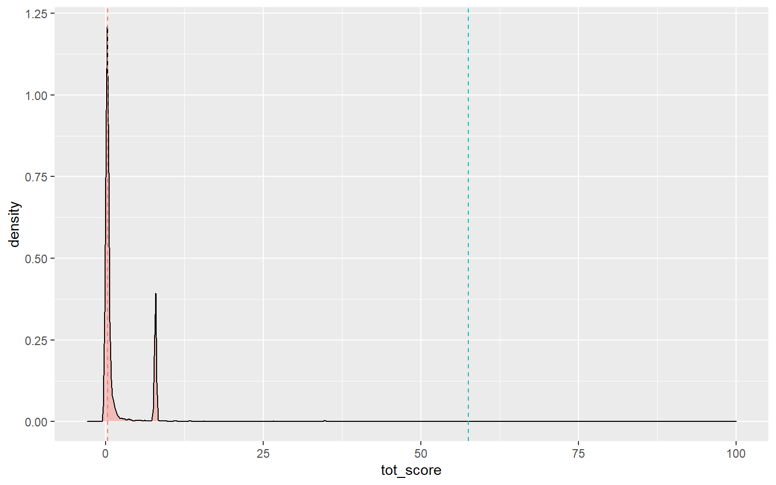
df <- df %>%
  mutate(influecer_score = if_else(tot_score >= 7.1 & is_retweet == "FALSE"
                                   ,"influencer","no influencer"))
6.3 The Topic Modeling and the speicification for STM!
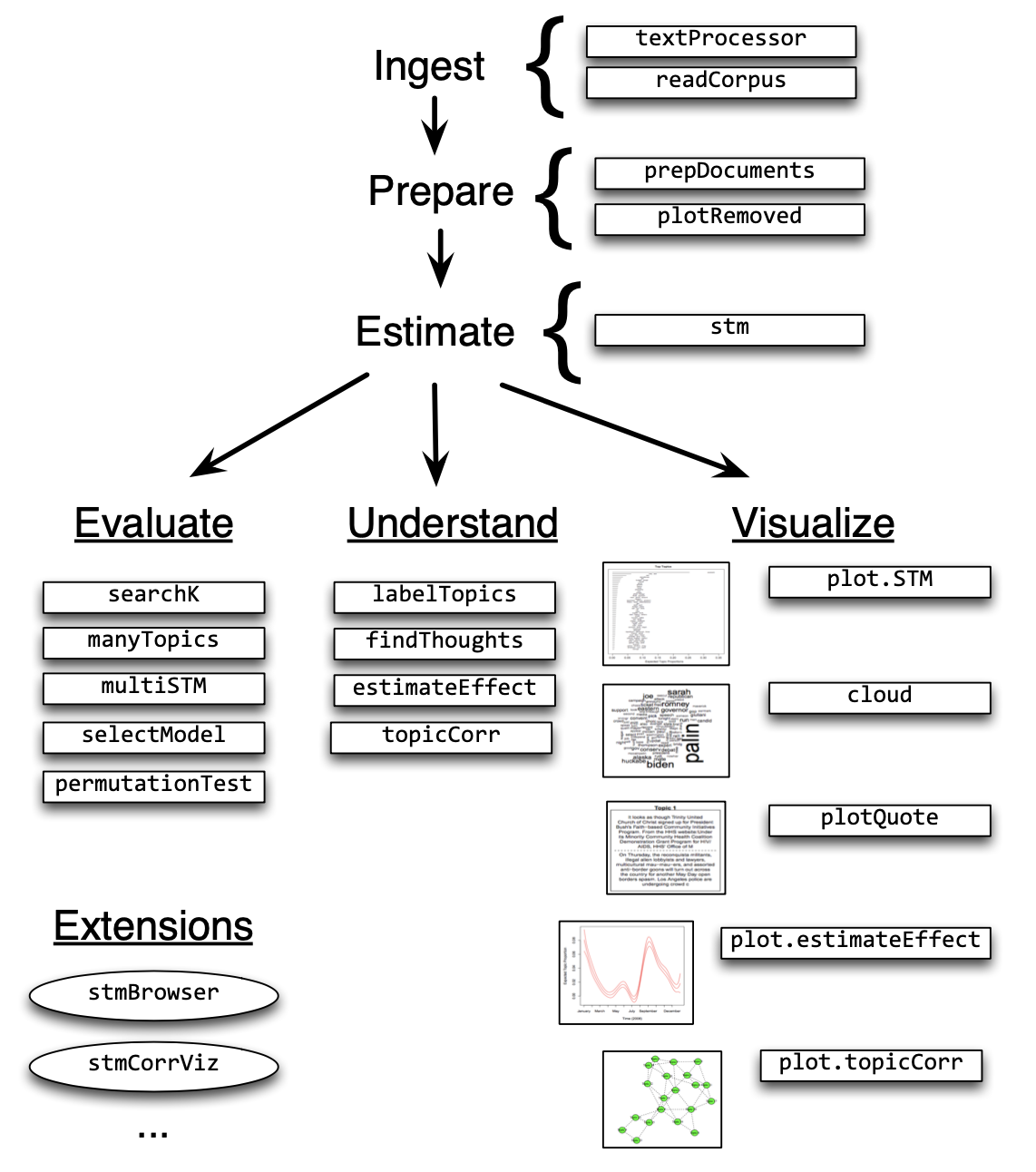
The Structural Topic Model allows researchers to flexibly estimate a topic model that includes document-level metadata. Estimation is accomplished through a fast variational approximation. The stm package provides many useful features, including rich ways to explore topics, estimate uncertainty, and visualize quantities of interest. Below an stm Workflow example!
Pre-processing text content
The most common processing steps are stemming (reducing words to their root form), dropping punctuation and stop word removal (e.g., the, is, at)
library(stm)

processed <- textProcessor(df$text, metadata = df)
## Building corpus...
## Converting to Lower Case...
## Removing punctuation...
## Removing stopwords...
## Removing numbers...
## Stemming...
## Creating Output...out <- prepDocuments(processed$documents, processed$vocab, processed$meta)## Removing 1432 of 6168 terms (1432 of 90615 tokens) due to frequency
## Removing 3 Documents with No Words
## Your corpus now has 4980 documents, 4736 terms and 89183 tokens.docs <- out$documents
vocab <- out$vocab
meta <- out$metaThen, prepDocuments() was used to structure and index the data for usage in the structural topic model. The object should have no missing values. Low frequency words can be removed using the ‘lower.thresh’ option. See ?prepDocuments for more information.
6.4 Estimating the structural topic model
The function selectModel() assists the user in finding and selecting a model with desirable properties in both semantic coherence and exclusivity dimensions (e.g., models with average scores towards the upper right side of the plot)
poliblogSelect <- selectModel(out$documents, out$vocab, K=5,
                              prevalence= ~ influecer_score + (tot_score) + s(created_at),
                              max.em.its=5, data=meta, runs=5, seed=123, init.type="LDA")
## Casting net
## 1 models in net
## 2 models in net
## 3 models in net
## 4 models in net
## 5 models in net
## Running select models
## 1 select model run
## Beginning LDA Initialization
## .....................................................................................................
## Completed E-Step (1 seconds).
## Completed M-Step.
## Completing Iteration 1 (approx. per word bound = -6.098)
## .....................................................................................................
## Completed E-Step (1 seconds).
## Completed M-Step.
## Completing Iteration 2 (approx. per word bound = -6.086, relative change = 1.912e-03)
## .....................................................................................................
## Completed E-Step (1 seconds).
## Completed M-Step.
## Completing Iteration 3 (approx. per word bound = -6.076, relative change = 1.656e-03)
## .....................................................................................................
## Completed E-Step (1 seconds).
## Completed M-Step.
## Completing Iteration 4 (approx. per word bound = -6.062, relative change = 2.289e-03)
## .....................................................................................................
## Completed E-Step (0 seconds).
## Completed M-Step.
## Model Terminated Before Convergence ReachedThe plotModels function calculates the average across all topics for each run of the model and plots these by labeling the model run with a numeral. Often users will select a model with desirable properties in both dimensions (i.e., models with average scores towards the upper right side of the plot)!
Let’s look at the results !!
poliblogPrevFit <- poliblogSelect$runout[[1]]
topicQuality(model=poliblogPrevFit, documents=docs)
## [1] -167.10844 -102.61500 -16.11098 -150.77353 -119.27140
## [1] 9.442292 9.212997 9.944086 9.395768 9.401330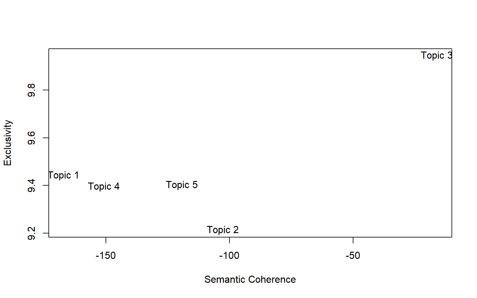
plot(poliblogPrevFit, type="perspectives", topics=c(1,3))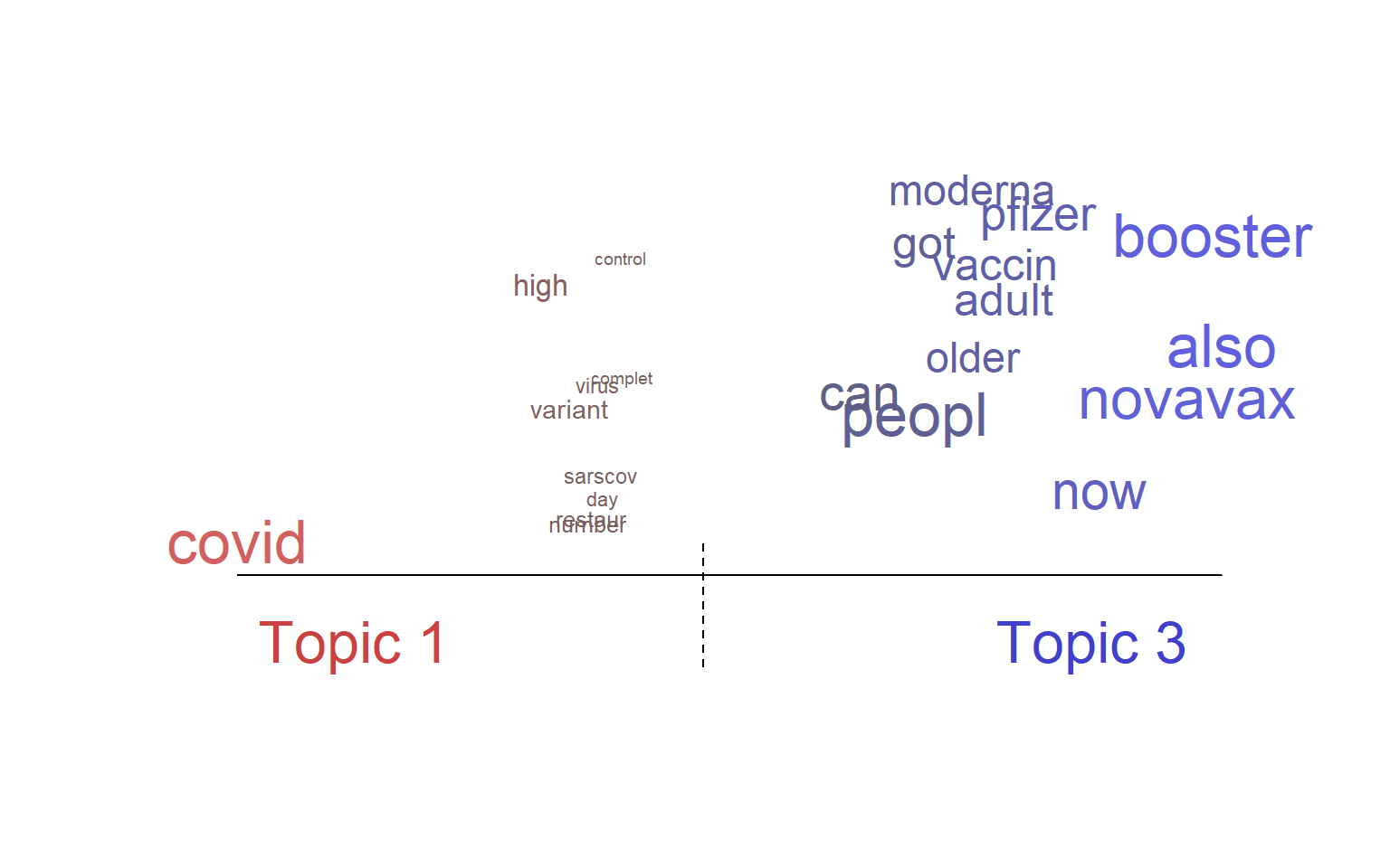
Words in topic
plot(poliblogPrevFit, type="labels", topics=c(1,2,3))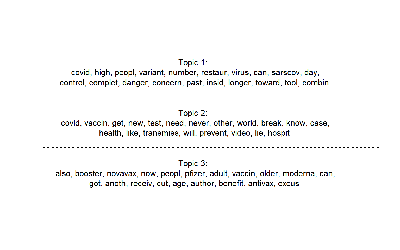
Words topics probabilities Plots
Plots the beta distribution of words per Topic
df_beta <- tidy(poliblogPrevFit)

df_beta %>%
  group_by(topic) %>%
  top_n(10, beta) %>%
  ungroup() %>%
  arrange(topic, -beta) %>%
  mutate(term = fct_reorder(term, beta)) %>%
  ggplot(aes(term, beta, fill = factor(topic))) +
  geom_col(show.legend = FALSE) +
  facet_wrap(~ topic, scales = "free_y", ncol = 3) +
  coord_flip() +
  scale_x_reordered() +
  labs(x = NULL, y = expression(beta),
         title = "Word probabilities for each topic",
         subtitle = "Words belonging to different topics")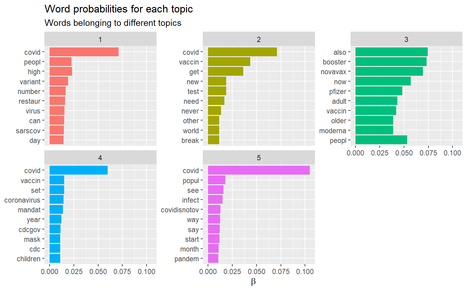
td_gamma <- tidy(poliblogPrevFit, matrix = "gamma",document_names = rownames(df))

td_gamma %>%
  group_by(topic) %>%
  top_n(10, gamma) %>%
  ggplot(aes(x = reorder(document, -gamma), y = gamma, color = factor(topic))) +
  facet_wrap(~ topic, scales = "free", ncol = 3) +
  geom_point(show.legend = FALSE, size = 1, alpha = 0.8) +
  coord_flip() +
  labs(x = "",
       y = "gamma\n(~ affiliation with topics)")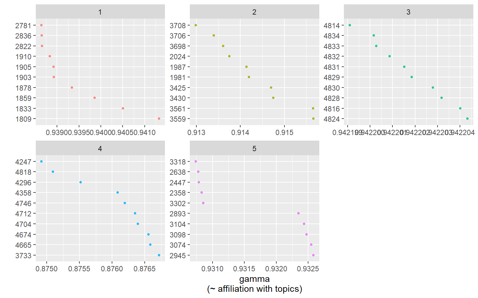
6.5 Estimating metadata/topic relationships
Estimating the relationship between metadata and topics is a core feature of the stm package. This function explores how prevalence of topics varies across documents according to the dataset covariates (metadata). The estimateEffect can calculate uncertainty in several ways. The default is “Global”, which will incorporate estimation uncertainty of the topic proportions into the uncertainty estimates using the method of composition.
out$meta$source <- as.factor(out$meta$source)

prep <- estimateEffect(1:5 ~ influecer_score,
                       poliblogPrevFit, meta=out$meta,
                       uncertainty="Global")

summary(prep)
##
## Call:
## estimateEffect(formula = 1:5 ~ influecer_score, stmobj = poliblogPrevFit,
## metadata = out$meta, uncertainty = "Global")
##
##
## Topic 1:
##
## Coefficients:
## Estimate Std. Error t value Pr(>|t|)
## (Intercept) 0.19999 0.02910 6.872 7.12e-12 ***
## influecer_scoreno influencer -0.01324 0.02936 -0.451 0.652
## ---
## Signif. codes: 0 '***' 0.001 '**' 0.01 '*' 0.05 '.' 0.1 ' ' 1
##
##
## Topic 2:
##
## Coefficients:
## Estimate Std. Error t value Pr(>|t|)
## (Intercept) 0.25525 0.02747 9.291 <2e-16 ***
## influecer_scoreno influencer -0.05211 0.02731 -1.908 0.0565 .
## ---
## Signif. codes: 0 '***' 0.001 '**' 0.01 '*' 0.05 '.' 0.1 ' ' 1
##
##
## Topic 3:
##
## Coefficients:
## Estimate Std. Error t value Pr(>|t|)
## (Intercept) 0.04121 0.03166 1.302 0.193
## influecer_scoreno influencer 0.14353 0.03196 4.491 7.26e-06 ***
## ---
## Signif. codes: 0 '***' 0.001 '**' 0.01 '*' 0.05 '.' 0.1 ' ' 1
##
##
## Topic 4:
##
## Coefficients:
## Estimate Std. Error t value Pr(>|t|)
## (Intercept) 0.228728 0.028379 8.060 9.48e-16 ***
## influecer_scoreno influencer -0.006373 0.028279 -0.225 0.822
## ---
## Signif. codes: 0 '***' 0.001 '**' 0.01 '*' 0.05 '.' 0.1 ' ' 1
##
##
## Topic 5:
##
## Coefficients:
## Estimate Std. Error t value Pr(>|t|)
## (Intercept) 0.27478 0.02874 9.561 <2e-16 ***
## influecer_scoreno influencer -0.07173 0.02889 -2.483 0.0131 *
## ---
## Signif. codes: 0 '***' 0.001 '**' 0.01 '*' 0.05 '.' 0.1 ' ' 1Plotting metadata/topic relationships, as the ability to estimate the relationships across the selected variable!!
plot(prep, covariate="influecer_score", topics = c(1:5), model=poliblogPrevFit,
     method="difference",
     cov.value1 = "influencer", cov.value2 = "no influencer",
     xlab = "topics less influencer ... topics more Influencer",
     labeltype = "custom",
     main = "Influencer topics appartenance",
     xlim=c(-0.20, 0.25))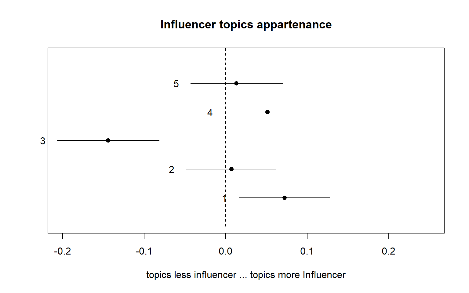
All the materials used will be available on my GitHub page, or on my BlogPage
Do not hesitate to contact me for further information s.pirri@regulatorypharmanet.com
#content{
    max-width:1720px;
}