Topic modeling and tweets text analysis

Unsupervised classification methodology for text analysis

2020-11-15 189 min read

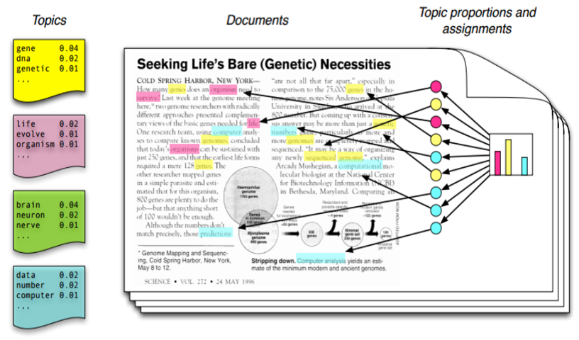
Topic modeling is a methodology for unsupervised classification, similar to the clustering methods numeric data, which finds natural groups of items across a set of documents. Topic Modeling is used to discover “latent” topics in a given selection of documents. Topic models are particularly common in text mining to unearth hidden semantic structures in textual data.Topic models are also referred to as probabilistic topic models, which refers to statistical algorithms for discovering the latent semantic structures of an extensive text body One of the most popular topic models is latent Dirichlet allocation (LDA) Blei et al. 2003.

LDA is a particularly popular method for fitting a topic model. It treats each document as a mixture of topics, and each topic as a mixture of words. This allows documents to “overlap” each other in terms of content, rather than being separated into discrete groups, in a way that mirrors typical use of natural language.

Latent Dirichlet allocation is one of the most common algorithms for topic modeling. Without diving into the math behind the model, we can understand it as being guided by two principles.

Every document is a mixture of topics. We imagine that each document may contain words from several topics in particular proportions. For example, in a two-topic model we could say “Document 1 is 90% topic A and 10% topic B, while Document 2 is 30% topic A and 70% topic B.”
Every topic is a mixture of words. For example, we could imagine a two-topic model of American news, with one topic for “politics” and one for “entertainment.” The most common words in the politics topic might be “President”, “Congress”, and “government”, while the entertainment topic may be made up of words such as “movies”, “television”, and “actor”. Importantly, words can be shared between topics; a word like “budget” might appear in both equally.

Structural Topic Model is a general framework for topic modeling with document-level covariate information, which can improve inference and qualitative interpretability by affecting topical prevalence, topic content, or both. The goal of the Structural Topic Model is to allow researchers to discover topics and estimate their relationships to document metadata where the outputs of the models can be used for hypothesis testing of these relationships. To do so, the stm package will be used.

For this tutorial, I will use data from the published article of Topic Modeling and User Network Analysis on Twitter during World Lupus Awareness Day. The original data consists of 4434 tweets scraped from Twitter using the rtweet API

library(readxl)
library(tm)
library(syuzhet)
library(tidytext)
library(tidyverse)
library(broom)
library(stm)
library(rmarkdown)
library(DT)
library(kableExtra)

theme_set(theme_light())

Reading and processing text data

The first step is load the dataset into R.

tweet_wLd <- read_excel("D:/R.studio/tweet_wld.xlsx")

Step 2: Clean the Text

tweet_wLd$text <- tolower(tweet_wLd$text)  # Make everything consistently lower case
tweet_wLd$text <- gsub("http.+ |http.+$", "", tweet_wLd$text)  # Remove links
tweet_wLd$text <- gsub("[[:punct:]]", "", tweet_wLd$text)  # Remove punctuation
tweet_wLd$text <- gsub("[ |\t]{2,}", "", tweet_wLd$text)  # Remove tabs
tweet_wLd$text <- gsub("amp", "", tweet_wLd$text)# "&" is "&amp"after punctuation removed
tweet_wLd$text <- gsub("^ ", "", tweet_wLd$text)  # Leading blanks
tweet_wLd$text <- gsub(" $", "", tweet_wLd$text)  # Lagging blanks
tweet_wLd$text <- gsub(" +", " ", tweet_wLd$text) # General spaces

tweet_wLd %>%
  select(user_id, text, created_at, retweet_count, source ) %>%
  datatable( class = 'cell-border stripe', rownames = FALSE)

Influencer score analysis

No golds standard measure is in place to measure a unique influencers score! However, in this paper Isabel Anger and Christian Kittl, briefly explain the basic functions and communication possibilities on Twitter offering in the context of social influence, a simple measure to scoring the influence across certain audience.

# Measure the influencer score across the users
tweet_wLd <- tweet_wLd %>%
  mutate(R_rt = retweet.score/statuses_count) %>%
  mutate(R_i = retweet.score/followers_count) %>%
  mutate(R_f = followers_count/friends_count) 

tweet_wLd <- tweet_wLd %>%
  mutate(tot_score = (tweet_wLd$R_f + tweet_wLd$R_i + tweet_wLd$R_rt)/3)

Let’s look at the influencers distribution

tweet_wLd %>%
ggplot(aes(x=tot_score, fill="#69b3a2")) +
    geom_density(adjust=1.5, alpha=.4) +
  geom_vline(aes(xintercept = mean(tot_score), col = "red",), linetype = "dashed") +
  geom_vline(aes(xintercept = median(tot_score), col = "blue",), linetype = "dashed") +
  xlim(-3, 100) +
  theme(legend.position = "none")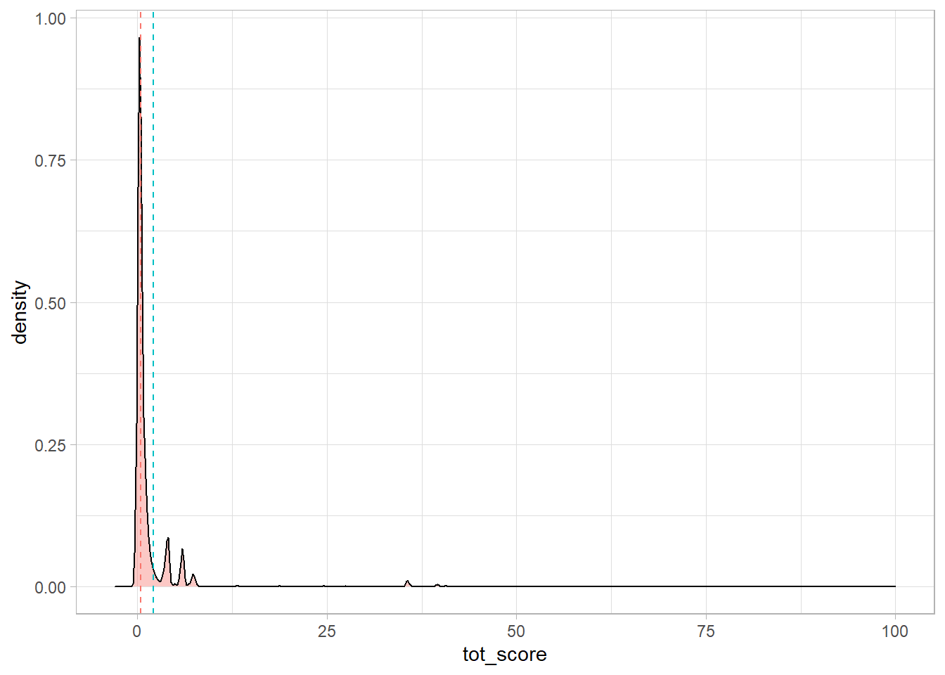

Quantiles are cut points dividing the range of a probability distribution into continuous intervals with equal probabilities, or dividing the observations in a sample in the same way.

quantiles <- quantile(tweet_wLd$tot_score, prob = c(0.10, 0.50, 0.85, 0.90))

quantiles

##        10%        50%        85%        90% 
## 0.09629133 0.38393131 2.11275964 3.99016979

#labeling the influencers
tweet_wLd <- tweet_wLd %>%
  mutate(influecer_score = if_else(tot_score >= 2.1 & is_retweet == "FALSE"
                                   ,"influencer","no influencer"))

The Topic Modeling and the speicification for STM!

The Structural Topic Model allows researchers to flexibly estimate a topic model that includes document-level metadata. Estimation is accomplished through a fast variational approximation. The stm package provides many useful features, including rich ways to explore topics, estimate uncertainty, and visualize quantities of interest. Below an stm Workflow example!

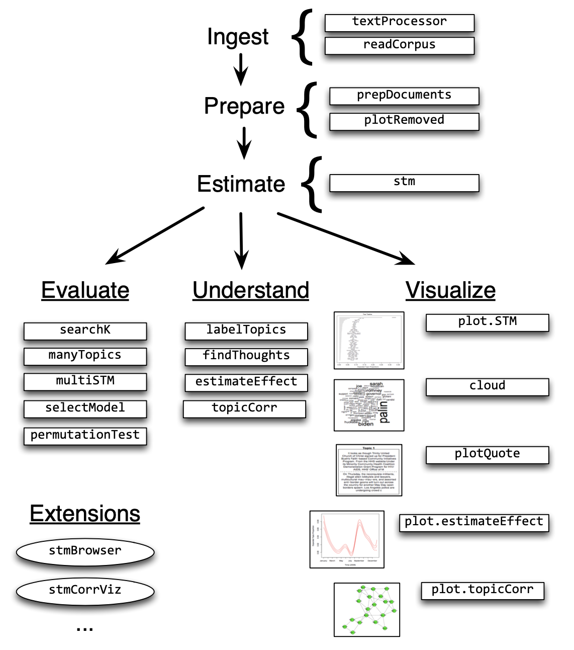
Find the optimal number of topics (k)

Accordinh with R. Arun, et al four metrics offer a solid way to select the most appropriate number of topics!

library(ldatuning)

text_corpus <- Corpus(VectorSource(tweet_wLd$text))
dtm <- DocumentTermMatrix(text_corpus)

result <- FindTopicsNumber(dtm = dtm , topics = seq(from = 4, to = 10, by = 1), 
                           metrics = c("Griffiths2004", "CaoJuan2009", "Arun2010", "Deveaud2014"),
                           method = "Gibbs",
                           control = list(seed = 123),
                           mc.cores = NA,
                           verbose = F)

result

##   topics Griffiths2004 CaoJuan2009 Arun2010 Deveaud2014
## 1     10     -155188.4   0.1933493 4919.912    2.191550
## 2      9     -156027.9   0.2122276 5015.536    2.176303
## 3      8     -158178.7   0.1906532 5075.728    2.306289
## 4      7     -158773.3   0.2151808 5208.194    2.253109
## 5      6     -162607.6   0.2594637 5418.124    2.250879
## 6      5     -165954.9   0.2707836 5560.213    2.290844
## 7      4     -169980.1   0.2861637 5740.716    2.281175

FindTopicsNumber_plot(result)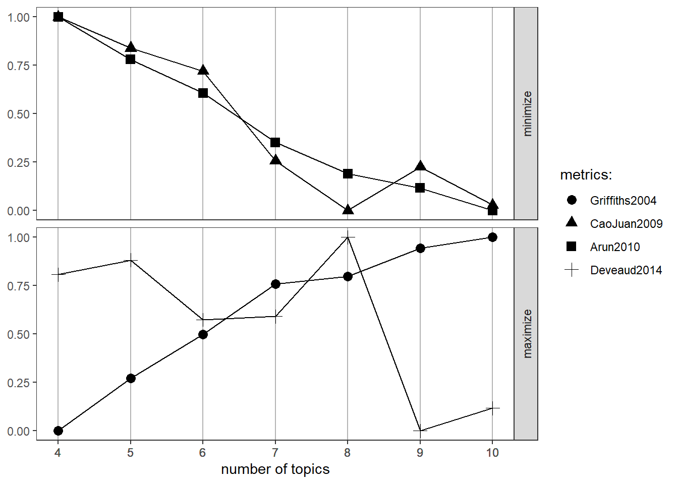

Pre-processing text content

The most common processing steps are stemming (reducing words to their root form), dropping punctuation and stop word removal (e.g., the, is, at)

processed <- textProcessor(tweet_wLd$text, metadata = tweet_wLd)

## Building corpus... 
## Converting to Lower Case... 
## Removing punctuation... 
## Removing stopwords... 
## Removing numbers... 
## Stemming... 
## Creating Output...

out <- prepDocuments(processed$documents, processed$vocab, processed$meta)

## Removing 646 of 1920 terms (646 of 20669 tokens) due to frequency 
## Your corpus now has 1342 documents, 1274 terms and 20023 tokens.

docs <- out$documents
vocab <- out$vocab
meta <- out$meta

Then, prepDocuments() was used to structure and index the data for usage in the structural topic model. The object should have no missing values. Low frequency words can be removed using the ‘lower.thresh’ option. See ?prepDocuments for more information.

plotRemoved(processed$documents, lower.thresh=seq(1,150))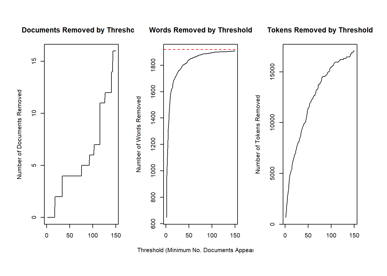

Estimating the structural topic model

The function selectModel() assists the user in finding and selecting a model with desirable properties in both semantic coherence and exclusivity dimensions (e.g., models with average scores towards the upper right side of the plot)

poliblogSelect <- selectModel(out$documents, out$vocab, K=7, 
                              prevalence= ~ influecer_score + (tot_score) + s(created_at),
                              max.em.its=50, data=meta, runs=20, seed=8159, init.type="LDA")

The plotModels function calculates the average across all topics for each run of the model and plots these by labeling the model run with a numeral. Often users will select a model with desirable properties in both dimensions (i.e., models with average scores towards the upper right side of the plot)!

plotModels(poliblogSelect)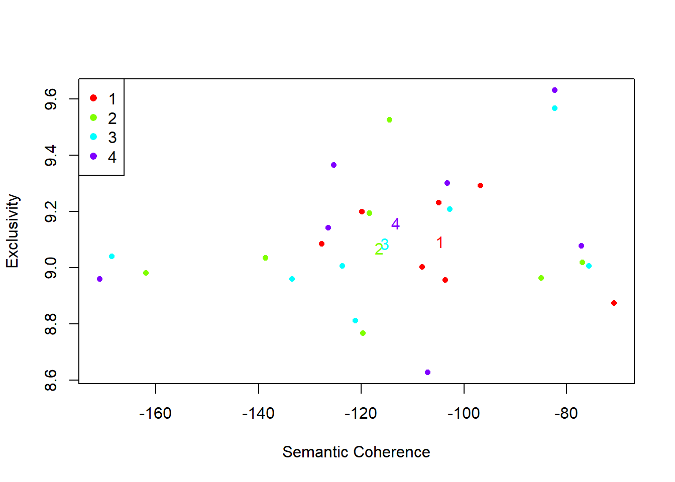

poliblogPrevFit <- poliblogSelect$runout[[2]]
topicQuality(model=poliblogPrevFit, documents=docs)

## [1] -114.55059  -76.93941 -119.75586  -84.99107 -138.72643 -118.46731 -161.98176
## [1] 9.527535 9.021080 8.767926 8.964424 9.036052 9.195909 8.982342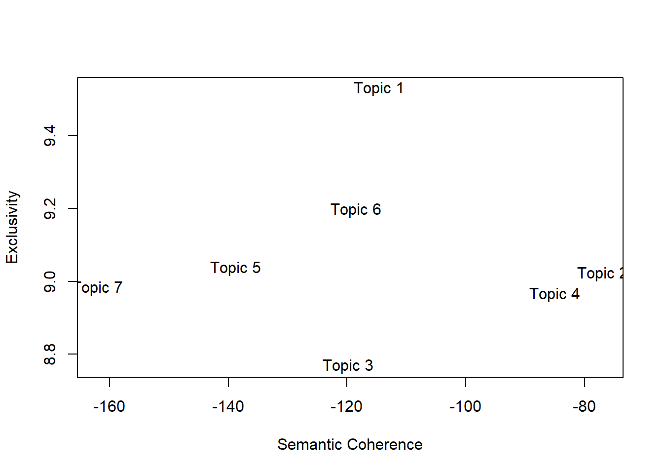

Understanding topics through words and example documents

Two approaches are describe for users to explore the topics that have been estimated. The first approach is to look at collections of words that are associated with topics. The second approach is to examine actual documents that are estimated to be highly associated with each topic.

plot(poliblogPrevFit, type="summary", xlim=c(0,.5))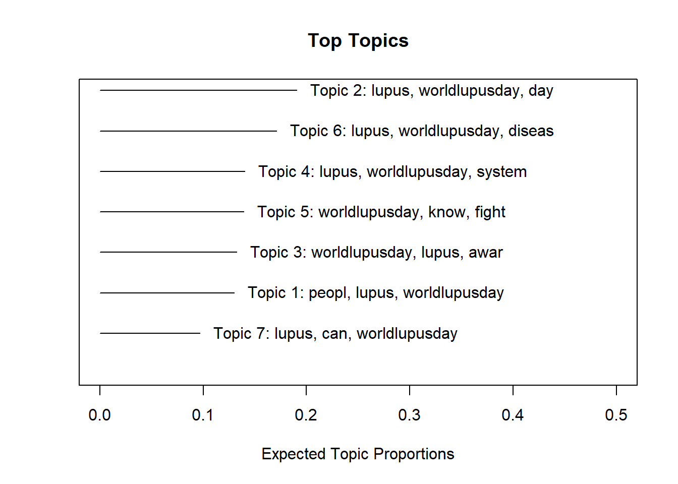

plot(poliblogPrevFit, type="labels", topics=c(1,2,3))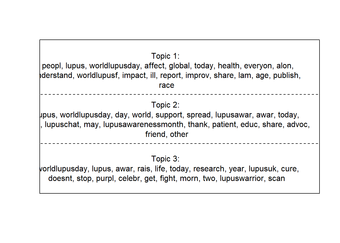

plot(poliblogPrevFit, type="hist")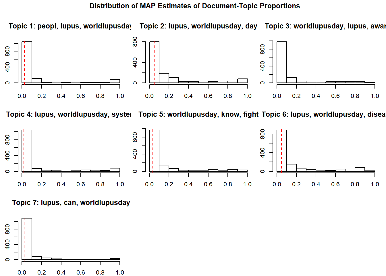

plot(poliblogPrevFit, type="perspectives", topics=c(1,3))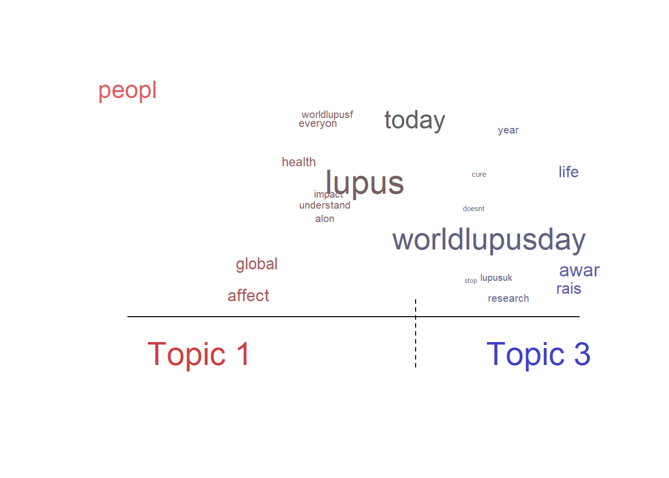

The findThoughts function print the text highly associated with each topic

findThoughts(poliblogPrevFit, texts = tweet_wLd$text, n = 1, topics=3)

## 
##  Topic 3: 
##       10 years misdiagnosed with chronic fatigue syndrome fibromyalgia and are things ok at home i spent my teen years in bed college wasnt accommodating about absences due to flares in 17 years i have never received adequate functional pain relief worldlupusday opioidcrisis

findThoughts(poliblogPrevFit, texts = tweet_wLd$text, n = 1, topics=1)

## 
##  Topic 1: 
##       lupus is a global health problem that affects people of all nationalities races ethnicities genders and ages 
## 
## during todays worldlupusday share the following expertled report published by worldlupusfed to improve the global understanding and impacts of lupus lam19

Words topics probabilities Plots

Plots the beta and (“gamma”) results

td_beta %>%
  group_by(topic) %>%
  top_n(10, beta) %>% 
  ungroup() %>%
  arrange(topic, -beta) %>%
  mutate(term = fct_reorder(term, beta)) %>%
  ggplot(aes(term, beta, fill = factor(topic))) +
  geom_col(show.legend = FALSE) +
  facet_wrap(~ topic, scales = "free_y", ncol = 3) +
  coord_flip() +
  scale_x_reordered() +
  labs(x = NULL, y = expression(beta),
         title = "Word probabilities for each topic",
         subtitle = "Words belonging to different topics")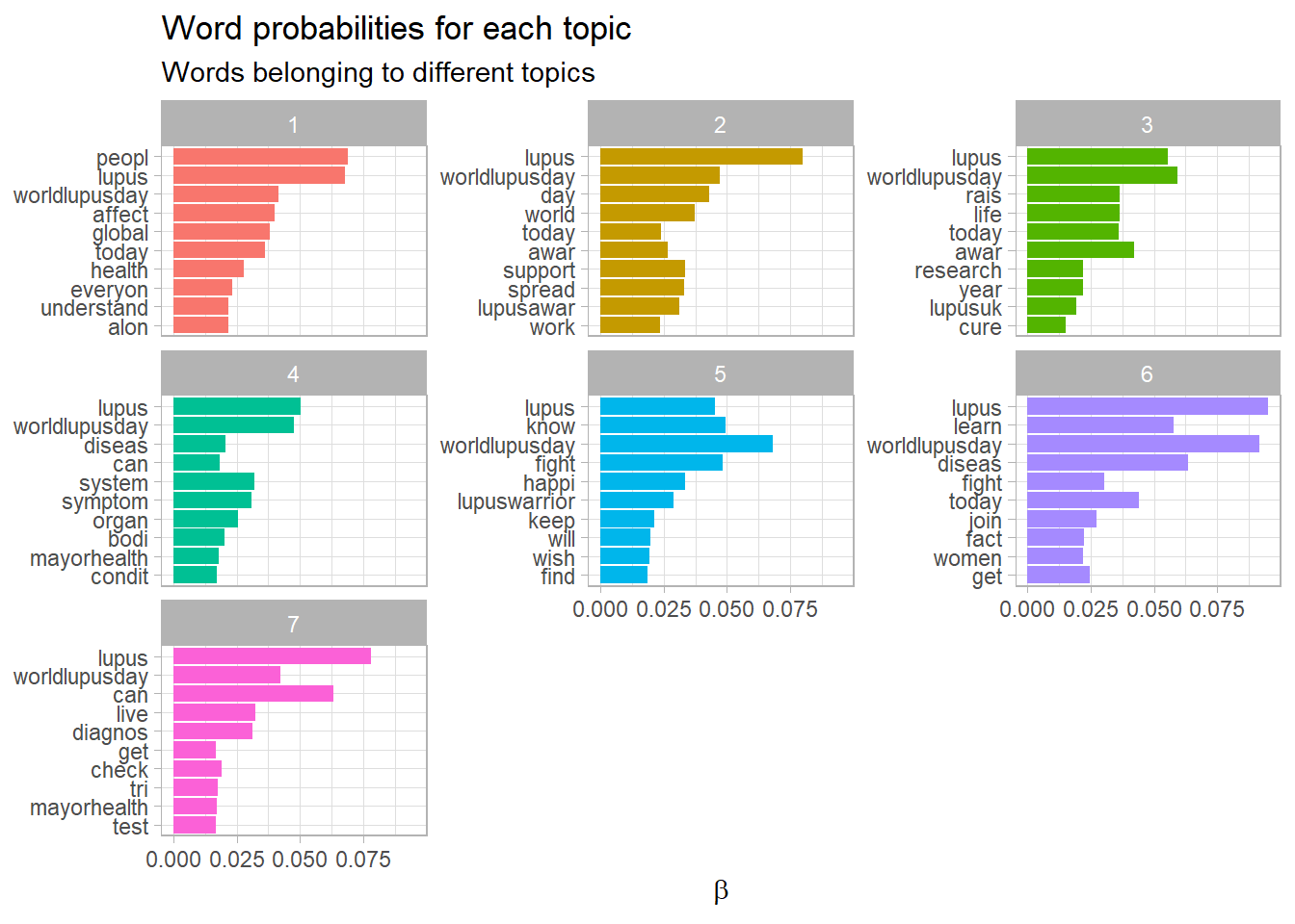

td_gamma %>%
  group_by(topic) %>%
  top_n(10, gamma) %>% 
  ggplot(aes(x = reorder(document, -gamma), y = gamma, color = factor(topic))) +
  facet_wrap(~ topic, scales = "free", ncol = 3) +
  geom_point(show.legend = FALSE, size = 1, alpha = 0.8) +
  coord_flip() +
  labs(x = "",
       y = "gamma\n(~ affiliation with topics)")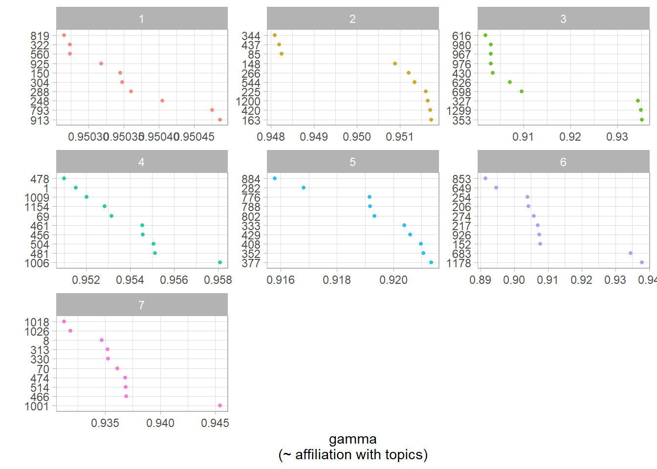

Estimating metadata/topic relationships

Estimating the relationship between metadata and topics is a core feature of the stm package. This function explores how prevalence of topics varies across documents according to the dataset covariates (metadata). The estimateEffect can calculate uncertainty in several ways. The default is “Global”, which will incorporate estimation uncertainty of the topic proportions into the uncertainty estimates using the method of composition.

out$meta$source <- as.factor(out$meta$source)

prep <- estimateEffect(1:7 ~ influecer_score, 
                       poliblogPrevFit, meta=out$meta, 
                       uncertainty="Global")

summary(prep)

## 
## Call:
## estimateEffect(formula = 1:7 ~ influecer_score, stmobj = poliblogPrevFit, 
##     metadata = out$meta, uncertainty = "Global")
## 
## 
## Topic 1:
## 
## Coefficients:
##                              Estimate Std. Error t value Pr(>|t|)   
## (Intercept)                   0.09020    0.03270   2.758  0.00589 **
## influecer_scoreno influencer  0.04987    0.03340   1.493  0.13566   
## ---
## Signif. codes:  0 '***' 0.001 '**' 0.01 '*' 0.05 '.' 0.1 ' ' 1
## 
## 
## Topic 2:
## 
## Coefficients:
##                              Estimate Std. Error t value Pr(>|t|)    
## (Intercept)                   0.07583    0.03219   2.356 0.018607 *  
## influecer_scoreno influencer  0.11365    0.03324   3.419 0.000646 ***
## ---
## Signif. codes:  0 '***' 0.001 '**' 0.01 '*' 0.05 '.' 0.1 ' ' 1
## 
## 
## Topic 3:
## 
## Coefficients:
##                              Estimate Std. Error t value Pr(>|t|)   
## (Intercept)                   0.09220    0.02950   3.125  0.00181 **
## influecer_scoreno influencer  0.04142    0.03069   1.349  0.17744   
## ---
## Signif. codes:  0 '***' 0.001 '**' 0.01 '*' 0.05 '.' 0.1 ' ' 1
## 
## 
## Topic 4:
## 
## Coefficients:
##                              Estimate Std. Error t value Pr(>|t|)    
## (Intercept)                   0.22384    0.03921   5.708 1.41e-08 ***
## influecer_scoreno influencer -0.08573    0.03943  -2.174   0.0299 *  
## ---
## Signif. codes:  0 '***' 0.001 '**' 0.01 '*' 0.05 '.' 0.1 ' ' 1
## 
## 
## Topic 5:
## 
## Coefficients:
##                              Estimate Std. Error t value Pr(>|t|)    
## (Intercept)                   0.12688    0.03198   3.968 7.63e-05 ***
## influecer_scoreno influencer  0.01381    0.03287   0.420    0.674    
## ---
## Signif. codes:  0 '***' 0.001 '**' 0.01 '*' 0.05 '.' 0.1 ' ' 1
## 
## 
## Topic 6:
## 
## Coefficients:
##                              Estimate Std. Error t value Pr(>|t|)    
## (Intercept)                   0.20432    0.03532   5.784 9.04e-09 ***
## influecer_scoreno influencer -0.04365    0.03600  -1.212    0.226    
## ---
## Signif. codes:  0 '***' 0.001 '**' 0.01 '*' 0.05 '.' 0.1 ' ' 1
## 
## 
## Topic 7:
## 
## Coefficients:
##                              Estimate Std. Error t value Pr(>|t|)    
## (Intercept)                   0.18744    0.03204   5.850 6.18e-09 ***
## influecer_scoreno influencer -0.09016    0.03218  -2.801  0.00516 ** 
## ---
## Signif. codes:  0 '***' 0.001 '**' 0.01 '*' 0.05 '.' 0.1 ' ' 1

Plotting metadata/topic relationships, as the ability to estimate the relationships across the selected variable!!

plot(prep, covariate="influecer_score", topics = c(1:7), model=poliblogPrevFit, 
     method="difference",
     cov.value1 = "influencer", cov.value2 = "no influencer",
     xlab = "topics less influencer ... topics more Influencer",
     labeltype = "custom",
     main = "Influencer topics appartenance",
     xlim=c(-0.20, 0.25))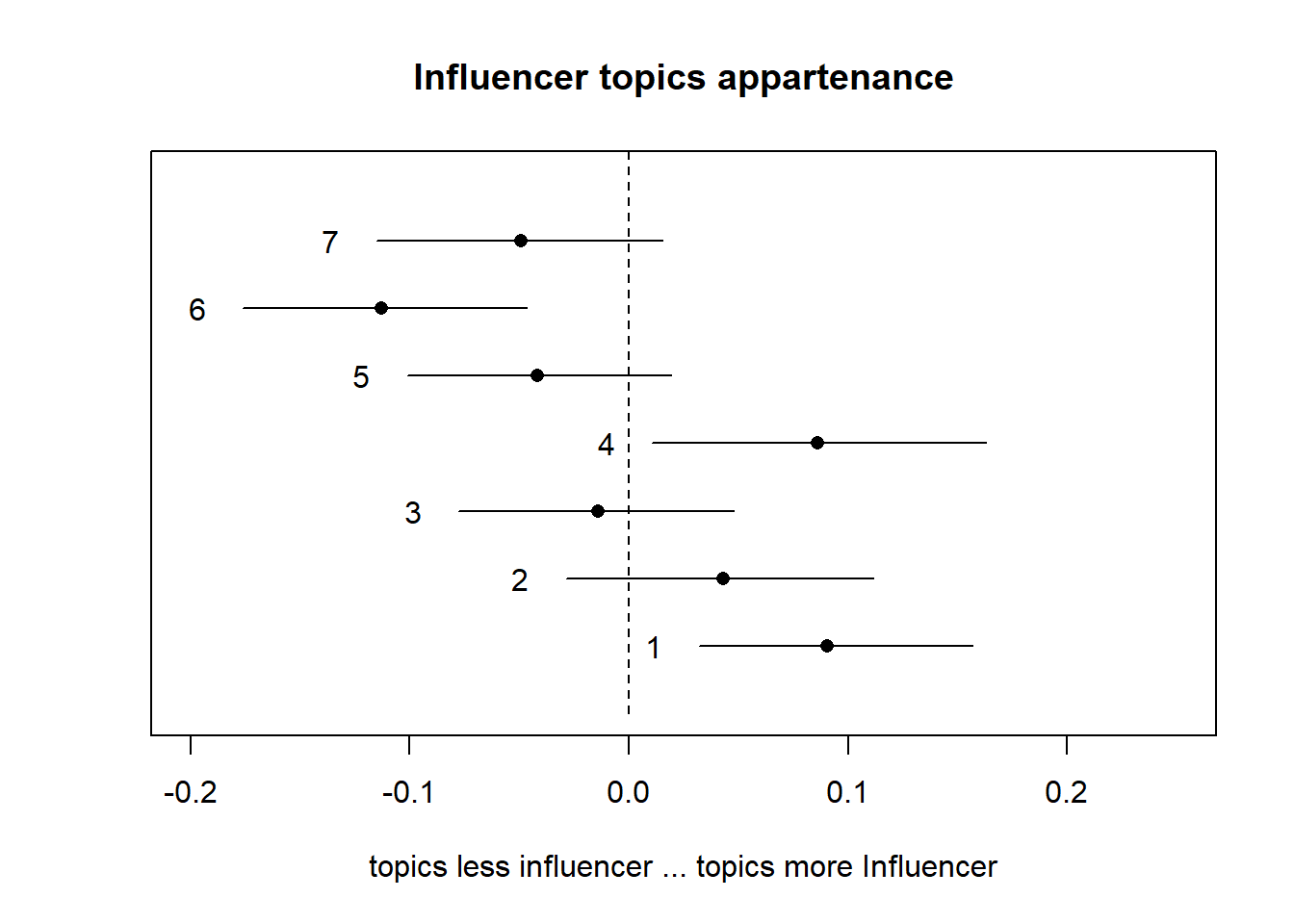

When the covariate of interest is binary, or users are interested in a particular contrast, the method = “difference” option will plot the change in topic proportion shifting from one specific value to another.

Salvatore Pirri

Value & Market Access Specialist - Research Affiliate in Health Economics

My research interests include Economics, machine learning and R programming.